#Understanding output

This page describes the output of each step and gives guidelines for tuning the settings. It is not exhaustive or definitive: imaging data varies a lot, so what worked for us might not work for you.

#Output layout

A typical run_pipeline run produces the following in rn_publish_dir (default ../results), next to the staged images (rn_image_dir) and deconvolved images (rn_decon_dir):

results/
├── images/                  # Staged images (rn_image_dir)
├── decon/                   # Deconvolved images (rn_decon_dir, dc_run)
├── flatfields/              # Flatfield models and evaluation plots
├── registration/            # Registration transforms and plots
├── masks/                   # Cellpose masks
├── rr__processed_images/    # Final images: unscaled/, scaled/, masks/
├── rr__features/            # measurements/ and cellprofiler/
├── rr__scaling/             # Scaling factors, see Scaling
├── rr__cellcrops/           # Single-cell crops
└── rr__qc/                  # QC report and per-well QC table

The folders without a prefix are a permanent cache; the rr__ folders are re-run by Nextflow when their inputs change and contain symbolic links into the work directory. See Re-running and caching.

Images, masks and most other per-field outputs follow the <plate>/<row>/<col>/ structure of the staged images. Channel numbers in all outputs are 0-indexed.

#Flatfield estimation

#Output

For every plate and channel, flatfield estimation writes a folder flatfields/<plate>/<plate>_ch<channel>/ with:

• profiles.npz and settings.json: the model, in the format used by BaSiCPy. The polynomial and PE modes use the same format, to keep the code consistent.
• PNG files to judge the quality of the fit, described below.

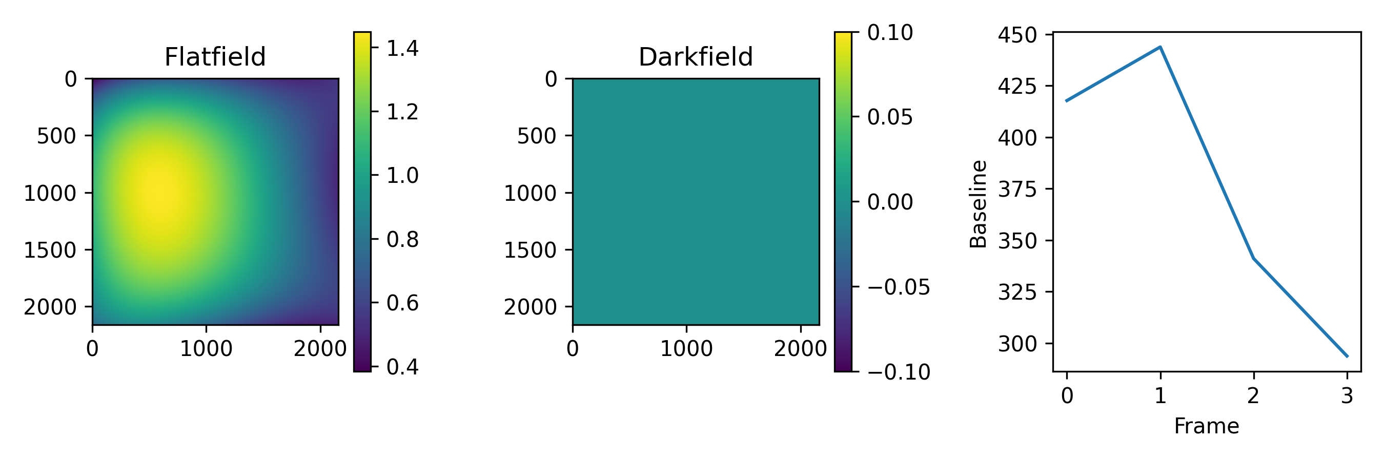
flat_and_darkfield.png shows the flatfield and the darkfield. The darkfield is not fitted and is always 0.

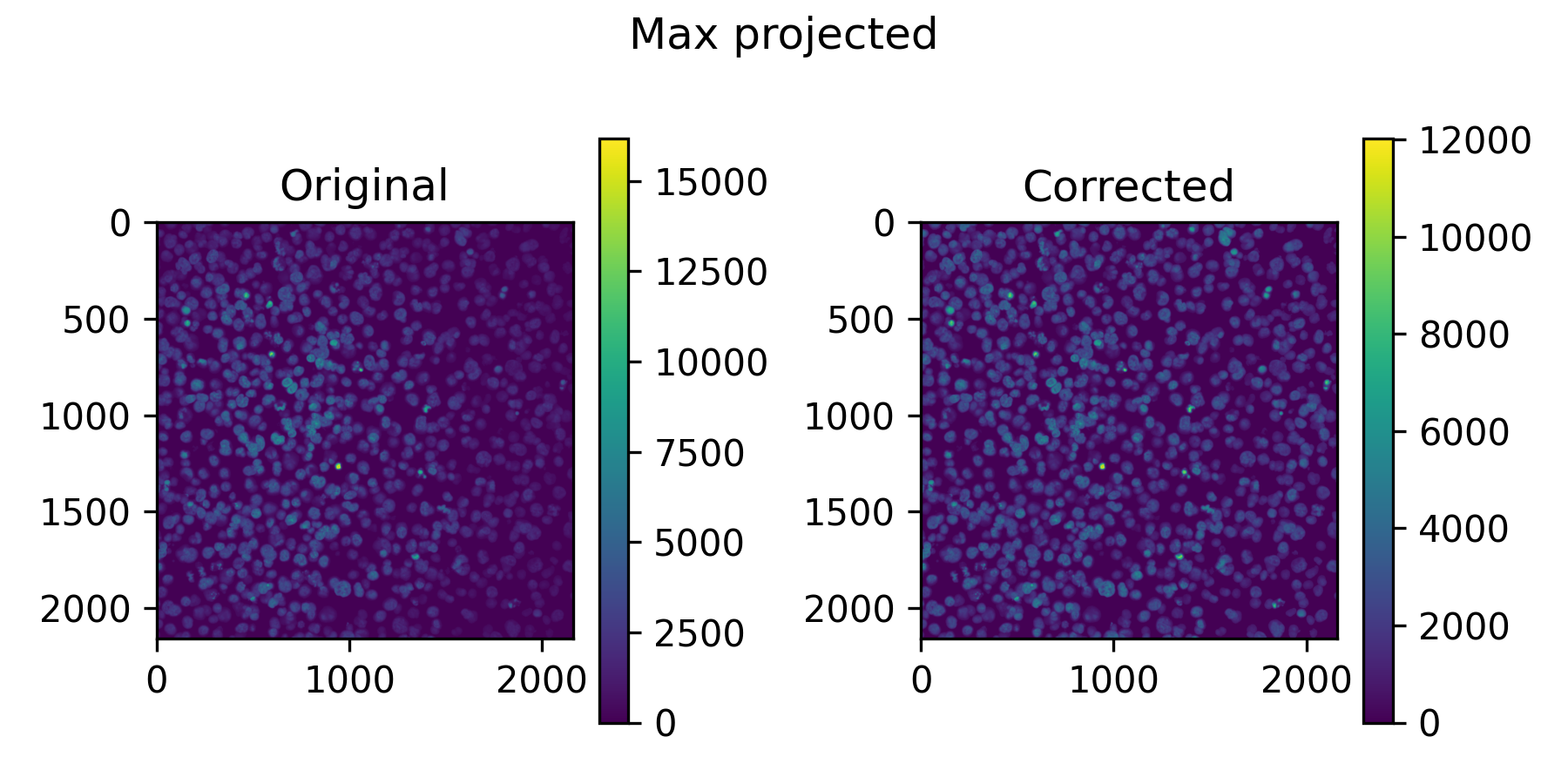
all_imgs_max_proj_pre_post.png shows a max projection of all training images, before and after applying the flatfield.

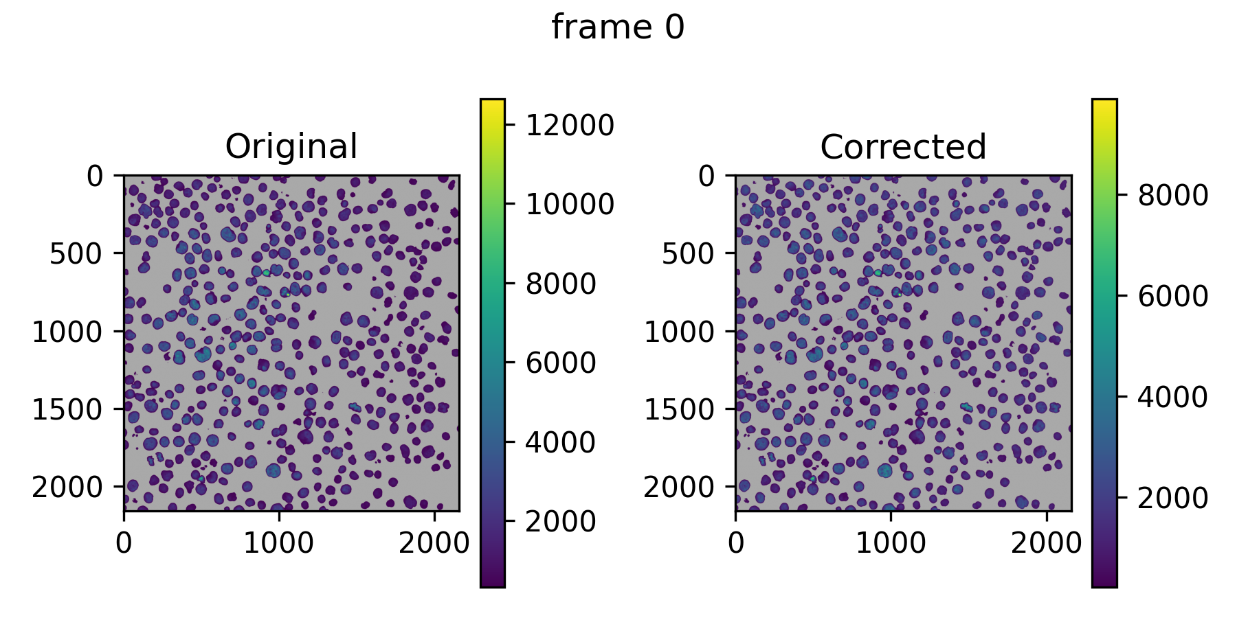
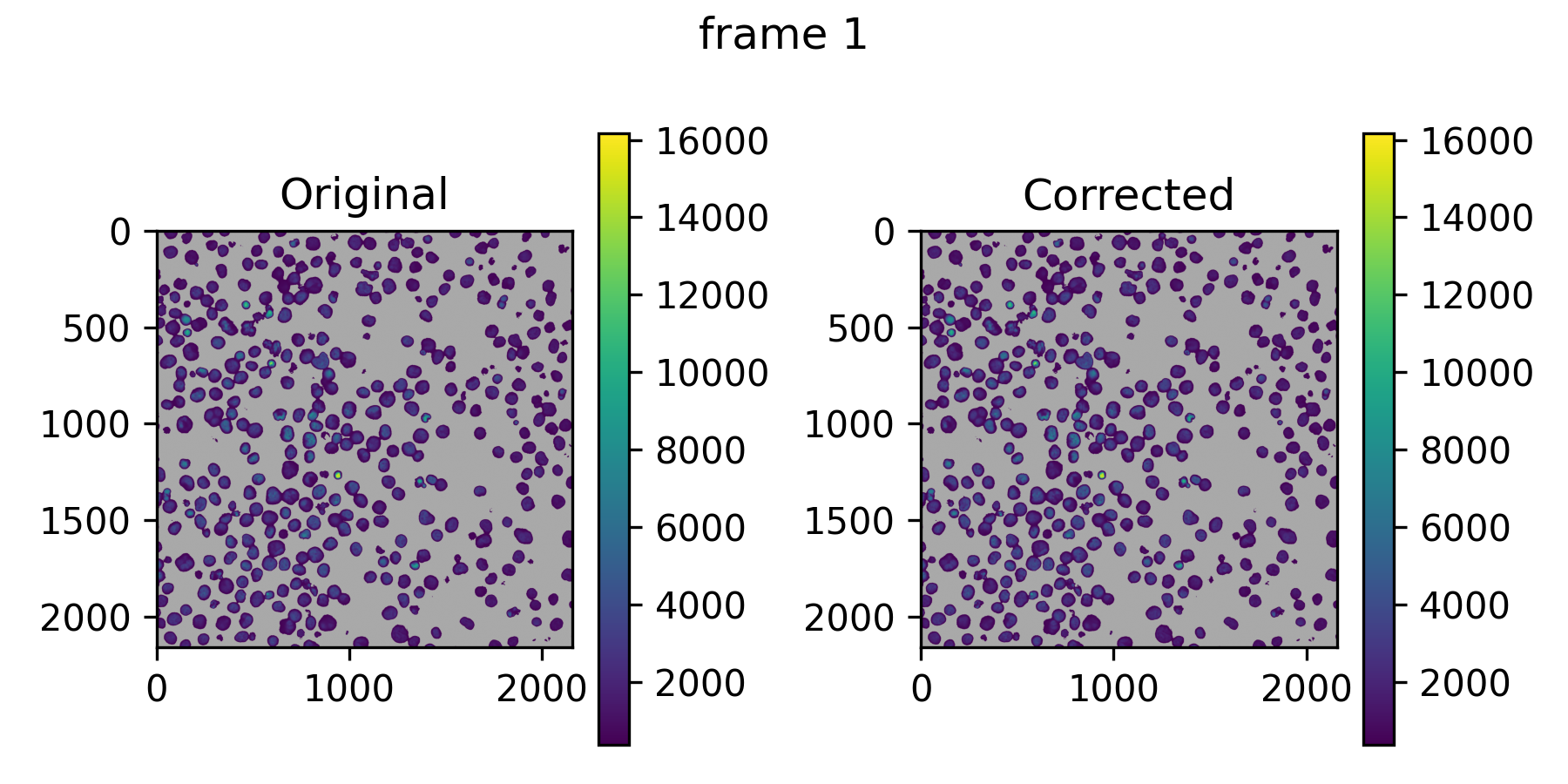
img<x>_pre_post.png shows the correction on the first training images. Grey pixels are background that was not used for training.

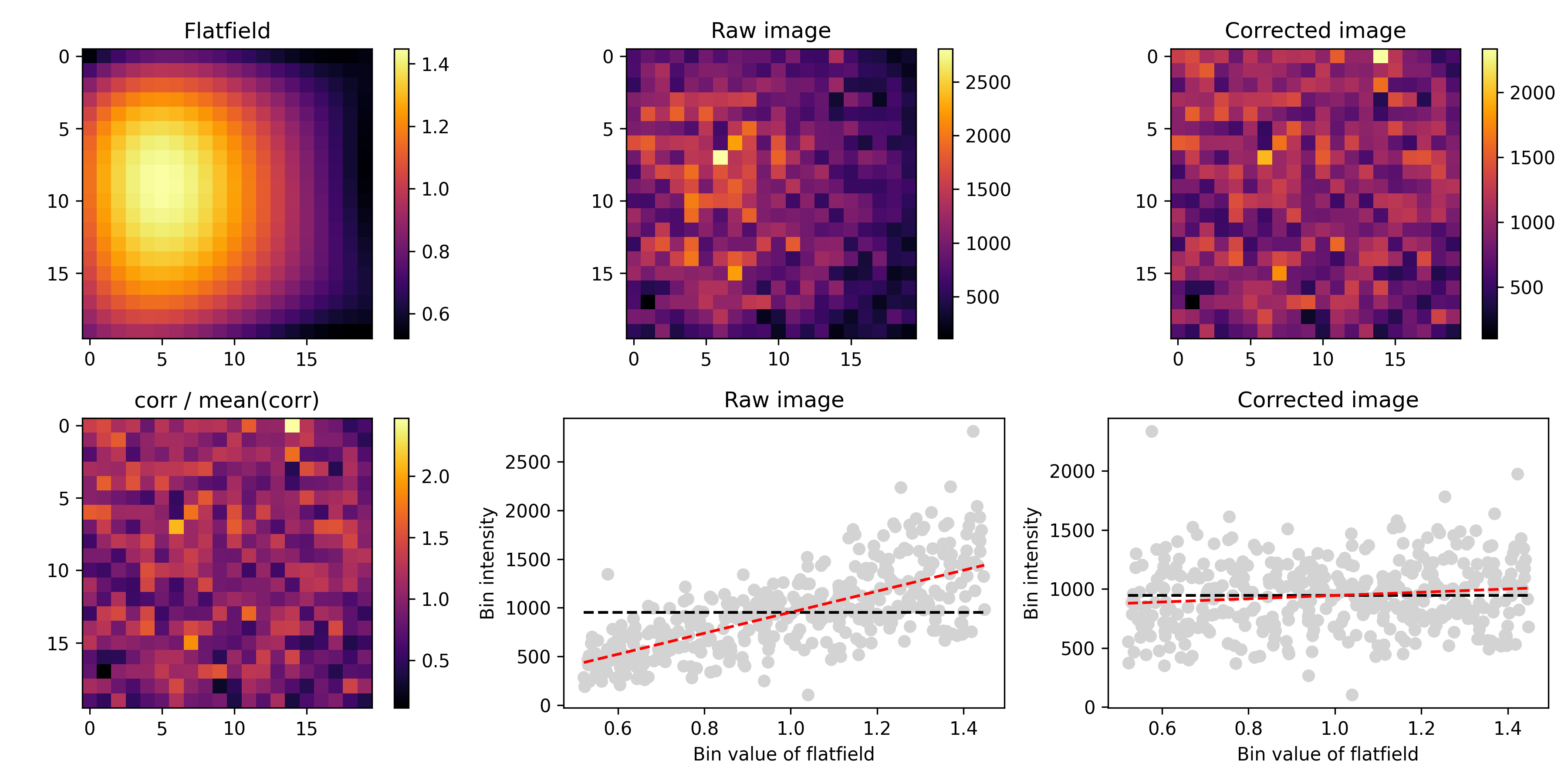
model_evaluation_nimg_<n>_nbin_<x>.png is the main evaluation plot, on randomly drawn test images that were not used for training (ff_nimg_test).

model_evaluation_pre_post_nimg_<n>_nbin_<x>.png shows the same as the pre_post plots, but on the test images. With ff_threshold = true there are also model_evaluation_thresh_<x>_... plots on the thresholded images.

In POLY mode with binned fitting (the default, see POLY), binned_fit.png compares the per-bin values the polynomial was fitted on with the fitted surface at those bins.

The flatfields also appear in the QC report.

#Modes

ff_mode selects how flatfields are estimated:

• POLY (default): fits a polynomial surface to the images.
• PE: takes the flatfield that Harmony calculated from the plate's Revity/PerkinElmer index file.
• BASICPY: fits BaSiCPy models on sampled images.

#POLY

With ff_degree 0 or below (the default), the polynomial has this form, which is the same approach Revity uses in Harmony:

1 + x + y + xy + x^2 + y^2 + x^3 + x^2*y + y^2*x + y^3 + x^4 + x^3*y + x^2*y^2 + y^3*x + y^4

Set ff_degree to fit a simpler or more complex full polynomial of that degree. We recommend a degree between 2 and 4. ff_use_ridge = true fits with cross-validated ridge regression instead of ordinary least squares.

The polynomial is not fitted on every pixel. The training images are divided into square bins of ff_bin_size pixels (default 20, which must evenly divide the image size), and the pixels of all training images that fall in a bin are pooled into one value, set by ff_bin_stat:

• mean (default): the smoothest fit.
• median: ignores bright outliers such as debris, but is noisier.
• trimmed: the mean after dropping ff_bin_trim (default 0.1) from each end, in between the two.
• none: the behaviour before v0.2.0, fitting on 4×4 block means of every image.

Every bin then counts equally in the fit, however many images contribute foreground there. In our testing this gave a closer fit to the true flatfield, and it uses far less memory. With ff_threshold = true, only foreground pixels are pooled. Bins with fewer than ff_bin_min_pixels (default 50) pooled pixels over all images are left out of the fit; if many bins are dropped, use more images, a larger ff_bin_size or a lower ff_bin_min_pixels.

#PE

Extracts the foreground flatfield from the Revity/PerkinElmer index file given in the manifest. Harmony doesn't always produce a flatfield, in which case this mode fails. With global flatfields, the index file of the first plate in the manifest is used.

#BASICPY

BaSiCPy is great, but seems to work best with very dense images, such as tissue sections. For Cell Painting or our tglow data it is harder to get reliable fits. See Sparsity and foreground selection below.

#Global flatfields

By default, a flatfield is fitted per plate and channel. With ff_global_flatfield = true, one flatfield per channel is fitted on images from all plates, which avoids a potential source of bias between plates. For multi-cycle data, a global flatfield is fitted per cycle, because cycles can have different base intensities that shift the flatfield, especially for dim signals.

Global flatfields are fitted for the ff_channels of the first plate in the manifest. Channels that other plates list in ff_channels but the first plate doesn't get no flatfield.

Because of the pipeline structure, global flatfields are stored under the reference plate as global_refplate_<plate>_ch<channel>, and copied to the folder of every plate. Even though they sit under one plate, they are trained on images from all plates.

#Sparsity and foreground selection

Depending on how strong the flatfield is, you may need many images for a good fit (ff_nimg, default 200). In sparse images, the background can dominate the fit, while the flatfield of the foreground signal is what matters. Options:

• ff_threshold = true fits only on the foreground pixels. The threshold is set by ff_threshold_mode, for POLY fitting and for the evaluation images:

  • otsu_log (default): an Otsu threshold on log-transformed intensities, the same method as the debris detection (sc_debris_method = "Otsu_log").
  • otsu: a two-class Otsu threshold divided by 4, the behaviour before v0.2.0. It is more lenient, but lets much of the background through when the signal is dim.

  In BASICPY mode, a plain Otsu mask is passed to BaSiCPy as fitting weights instead.

• ff_merge_n combines several images into one by max projection, to artificially increase the density of foreground signal. This can give more stable flatfields for very sparse images. ff_pseudoreplicates does something similar in memory, without reading more images.

In the example images, the pixels not used for fitting are grey, so you can see what goes into the model.

#Overriding flatfields

If a proper flatfield is hard to fit, but you have a better one from other data, copy it into the folder of the plate and channel you want to override. Because flatfields/ is a permanent cache, the pipeline will use your file. If you made it outside the pipeline, save it in the same format (profiles.npz and settings.json). You can create dummy files for the PNGs, for example with touch flat_and_darkfield.png, so the pipeline doesn't try to re-run anything.

#Deconvolution

Deconvolution (dc_run = true) writes the same <plate>/<row>/<col>/<field>.ome.tiff structure as the staged images to rn_decon_dir, with the deconvolved images. Channels without a PSF in the manifest's dc_psfs are not deconvolved, but go through the same 16-bit conversion described below. In 2D mode (rn_max_project = true without rn_hybrid), the deconvolved images are saved as max projections.

Deconvolution is done in 32-bit floats, but the images are stored as 16-bit integers to save space. To avoid clipping, the intensities of all channels are divided by dc_clip_max and multiplied by 65535. The default dc_clip_max of 327675 (5 × 65535) should prevent serious clipping in most cases, but make your own evaluation. It does lose some dynamic range at low intensities. You can set dc_clip_max = 65535 to keep the full dynamic range, at the risk of clipping if the input images were already close to the maximum intensity.

Compare before and after images in the QC report.

#Segmentation

Masks are stored as 16-bit TIFF files in masks/<plate>/<row>/<col>/, one per field for the cells and, if a nucleus channel is set, one for the nuclei:

<field>_cell_mask_d<cp_cell_size>_ch<channel>_cp_masks.tiff
<field>_nucl_mask_d<cp_nucl_size>_ch<channel>_cp_masks.tiff

In 3D and hybrid mode the masks are 3D. In 2D mode they are 2D, but saved as ZYX stacks regardless.

Only the reference plates are segmented, not later cycles, so you can only segment on stains in the first cycle. With deconvolution enabled, segmentation runs on the deconvolved images.

The main Cellpose settings are cp_cell_size, cp_nucl_size (the expected diameters in pixels), cp_cell_prob_threshold, cp_nucl_prob_threshold, cp_cell_flow_thresh and cp_nucl_flow_thresh. See the Cellpose documentation for what they mean. In rough order of importance:

1. Make sure the cell and nucleus sizes are right.
2. Tune the probability thresholds (between -6 and 6; higher gives tighter masks).
3. Tune the flow thresholds.
4. If you still get many false positives or negatives, set cp_min_cell_area and cp_min_nucl_area. By default these are derived from the cell and nucleus sizes, which may not work if cell sizes vary a lot.

3D segmentation can be slow. cp_downsample = 2 runs Cellpose on images downsampled 2 times in X and Y, and scales the masks back up to full resolution before saving. The sizes and minimum areas are adjusted automatically, so set them in terms of the original image. We recommend a whole number, and not going above 2 unless you have very high resolution images and simple, round cells. For complex shapes, full resolution may be better.

To evaluate the segmentation, inspect the processed images and masks in an image viewer such as Napari, or compare with a manually annotated gold standard. The pipeline has no built-in segmentation validation.

If you want to treat your cycles as separate plates, omit the registration manifest. This affects flatfield estimation and your CellProfiler pipeline, so in general we recommend separate runs with dedicated features for the extra cycles instead.

#Registration

Registration results are stored per field in registration/<reference plate>/<row>/<col>/:

• <field>.pickle: the translation that aligns each query cycle to the reference.
• <field>_<query plate>_refch<R>_qrych<Q>.png: a plot to evaluate the registration (rg_plot = true).
• registration_eval.tsv: per well, the correlation between the registration channels before and after registration (rg_eval = true).

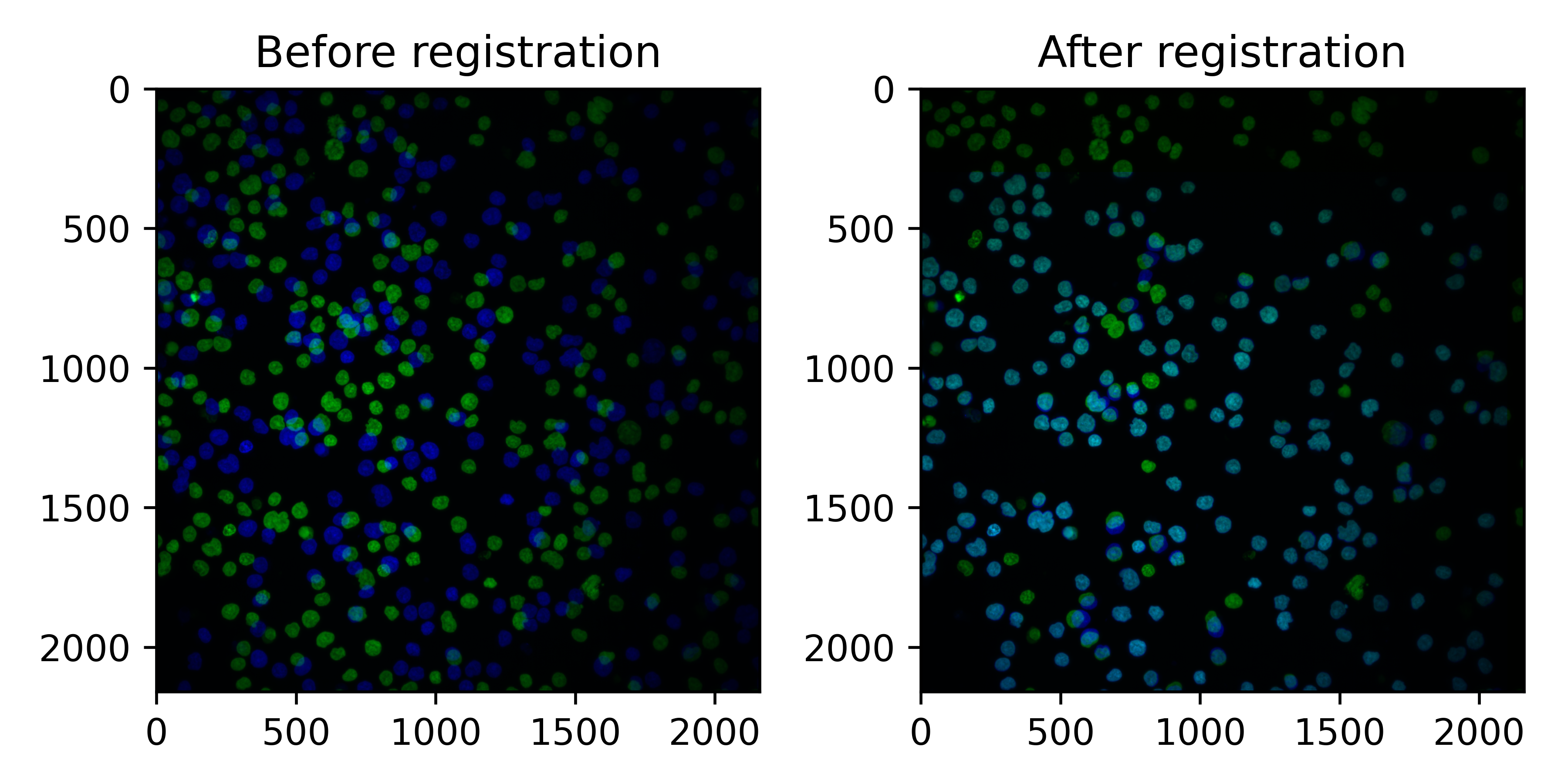
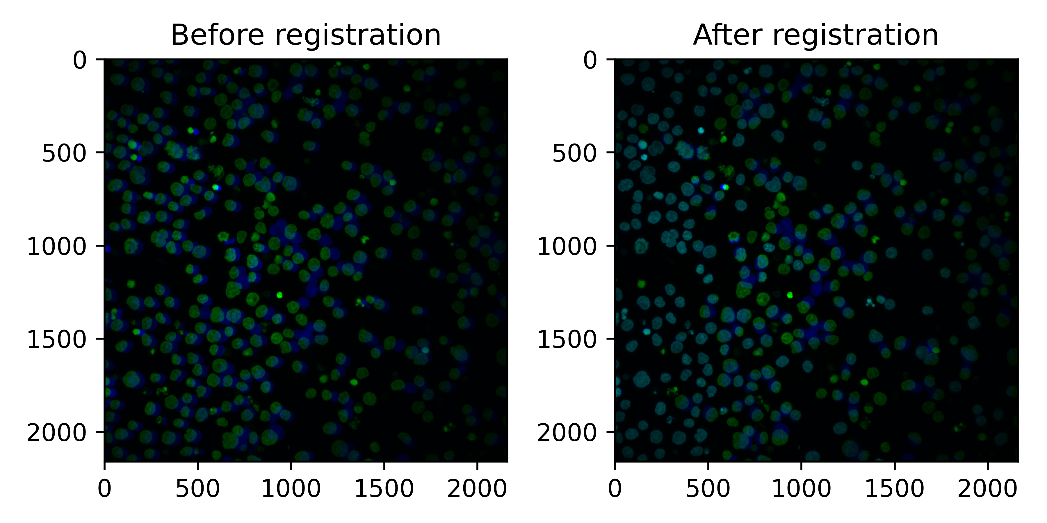
In the plots, the reference plate is green and the query cycle blue.

In the following example, registration worked well: some cells were lost (only green) but most cells align well.

In the next example, registration still worked, but more cells moved during the second cycle. These cells need to be removed downstream, but the ones that registered well can still be used.

Because individual cells can move between cycles, the pipeline also measures the correlation of the registration channels within each cell (ch<ref>_ch<query>__registration_corr in the measurements, one column per query cycle). Cells below sc_registration_thresh are excluded from scaling, and the QC report shows the worst and best aligning fields (see QC report). Use the same correlation to filter cells in downstream analysis.

#Processed images

Finalize combines everything into analysis-ready images in rr__processed_images/: the cycles merged, deconvolution and flatfields applied, registered, max projected (in 2D and hybrid mode), and demultiplexed into nuclear and non-nuclear channels for mask_channels.

Each image folder has a manifest.tsv per plate. unscaled/<plate>/channel_indices.tsv describes the final channels. It is published even when the unscaled images are not (sc_publish_unscaled = false):

Mask channels are appended at the end, named ... mask inclusive and ... mask exclusive. See Final channel numbers.

The processed images are easy to view in Napari, to check deconvolution and segmentation.

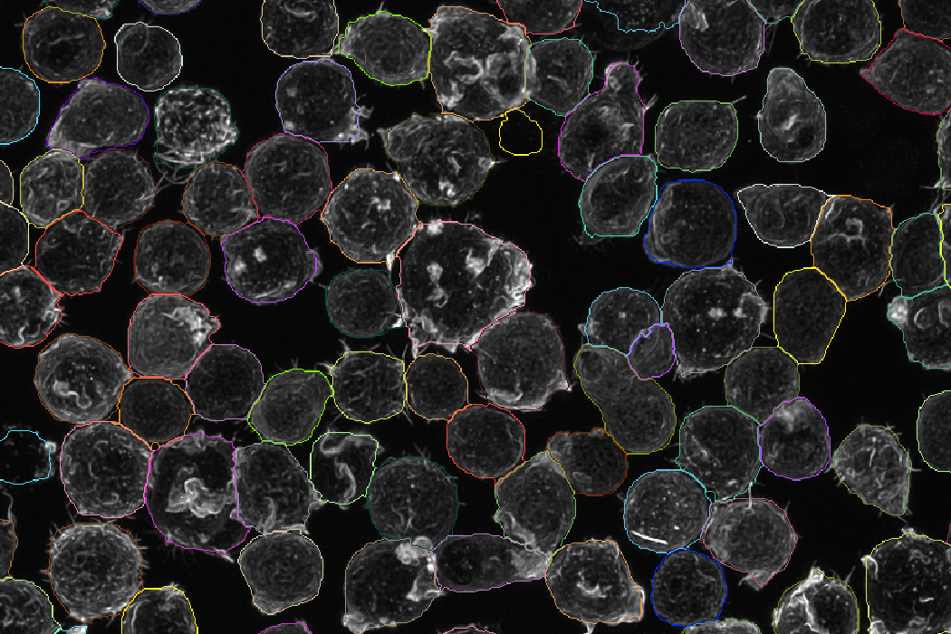
Example cell masks:

Example nucleus masks:

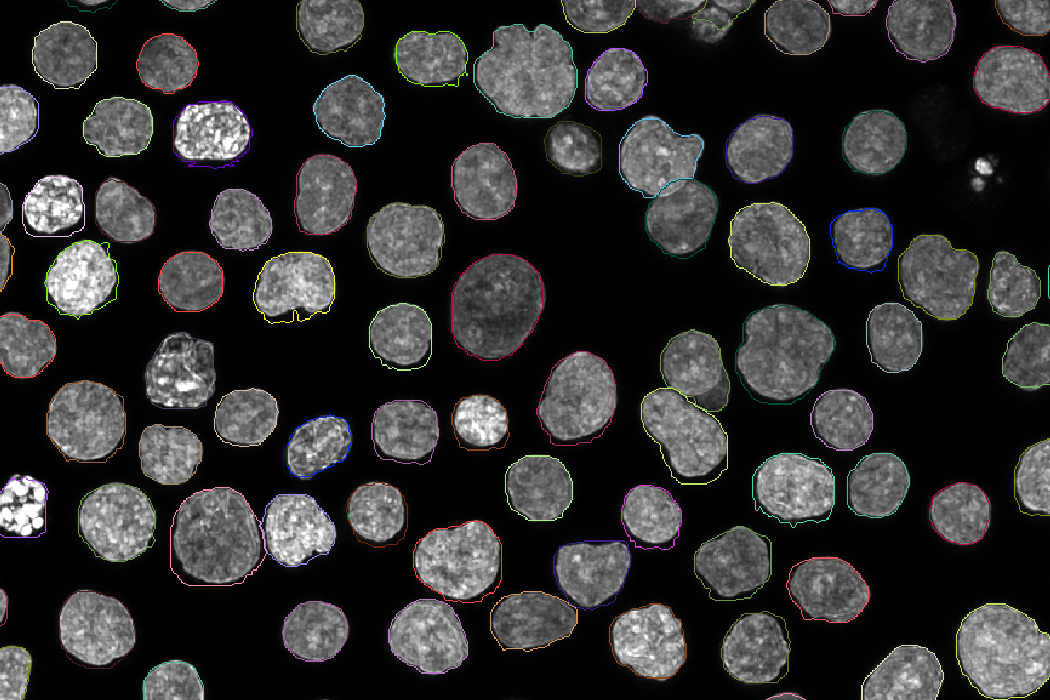
In hybrid mode, the 3D masks are max projected to get them into 2D. In some cases you may get nicer masks by segmenting the max projections directly, but the pipeline currently does not re-segment after max projection.

#Intensity measurements

With rn_cache_images = true, the pipeline measures every cell and image in the processed images. The measurements are used for scaling and the QC report, and are useful for your own QC. They are written per well to rr__features/measurements/<unscaled or scaled>/<plate>/<row>/<col>/:

• object_features.parquet: one row per cell, with columns ch<N>__<stat> (min, q5, q25, median, q75, q95, mean, max) for every final channel, measured in the cell or nucleus mask as set by the channel map. It also has each cell's position (centroid_x, centroid_y, centroid_z) and area, and for multi-cycle runs the registration correlation of each cell.
• image_features.parquet: one row per field, with background statistics (the pixels outside cells), thresholds, debris metrics and their debris-removed (_dbrm) variants. How debris is called is set by sc_debris_method and sc_cellmask_expansion, see QC report.

In 3D mode, the statistics are computed over all voxels of the stack rather than a projection, so scaling factors are fitted on the same intensities that rescaling is applied to. area is then a voxel count and centroid_z the cell's z position; for 2D input centroid_z is 0.

#Features

CellProfiler runs your own pipeline (cpr_pipeline_2d in 2D and hybrid mode, cpr_pipeline_3d in 3D mode) on each well. The images are staged for CellProfiler as one TIFF per field and channel:

<field>_<plate>_<well>_ch<channel>.tiff

where <plate> is the reference plate, <well> is written like A01, and <channel> is the final, 0-indexed channel number. The masks are in the same folder, with the names from Segmentation. See Configuring CellProfiler for how to set up the input modules and the export of your CellProfiler pipeline.

Output, in rr__features/cellprofiler/:

The aggregation (cpr_run_concat = true) reads the *_cell.txt and *_Image.txt files of each well. Every other file matching cpr_child_pattern is treated as a sub-object and merged onto its parent cell using the cpr_parent_col column (default Parent_cell, written by CellProfiler's RelateObjects module). When a cell has several sub-objects, their values are combined with cpr_merge_strategy (mean, median or sum). Columns get a prefix per object (for example cell_), and every row gets plate, well and global cell and image ids.

The aggregation needs the zipped output; with cpr_no_zip = true, you get the full unzipped CellProfiler output instead and no aggregation.

#Cell crops

With rn_make_cellcrops = true, the pipeline cuts every cell out of the processed images (the scaled images when scaling is enabled). In rr__cellcrops/<plate>/<row>/<col>/:

• <field>.h5: an HDF5 file per field, with one group per cell. The masks are appended as the last channels.

rr__cellcrops/cellcrop_index.parquet holds the metadata of every cell in the run: its index in the HDF5 file, position, crop size, intensities, registration correlation and so on. Use it to index the crops from tglow-r or when sampling cells to train deep learning models. (The per-well metadata files it is built from stay in the work directory and are not published.)

Each crop is a square centred on the cell's centre of mass, just large enough to contain every pixel of the cell, so irregular cells get larger crops. Its side length is stored as diameter. Cells whose crop would extend past the edge of the field are skipped, as are fields with more than rn_max_per_field (default 1000) cells.

For multi-cycle runs, corr_<ref>_<query> is the correlation between the reference and query registration channels within the cell's nucleus (or the whole cell, if there is no nucleus mask), comparable to CellProfiler's per-object Pearson correlation.

#QC report

See QC report.